You've built a RAG system. Your embeddings work. The prototype queries your 10,000 documents in milliseconds. Then someone asks: "What happens when we have 100 million documents?"
That question—scale—is where the vector database landscape gets interesting. And confusing. There are now dozens of options, each claiming to be the right choice. The reality is more nuanced: different tools solve different problems at different scales.
This is the guide I wish I had when I started building embedding-based systems. We'll trace the evolution from research libraries to production databases, understand the tech that makes it work, and end with a practical framework for choosing what fits your actual needs.
The Origin: It Started With a Library
Before there were vector databases, there was FAISS.
Facebook AI Similarity Search (FAISS) launched in 2017 as an open-source library—not a database, but a set of algorithms for finding similar vectors efficiently. It solved a fundamental problem: brute-force search through millions of high-dimensional vectors is computationally expensive. FAISS introduced optimized implementations of approximate nearest neighbor (ANN) algorithms that traded perfect accuracy for dramatic speed improvements.
The key insight: you don't need to find the exact nearest neighbor. Finding a very good approximate match is usually sufficient for real-world applications, and it's orders of magnitude faster.
FAISS remains important today—not as something you use directly, but as the foundation many vector databases build upon. Milvus, Vearch, and others incorporate FAISS algorithms under the hood. Understanding that FAISS is a library, not a database, helps clarify the landscape: it provides the search algorithms, but not the storage, replication, or query APIs that production systems need.
The Breakthrough: HNSW and Graph-Based Search
The algorithm that powers most modern vector databases is HNSW—Hierarchical Navigable Small World graphs. It sounds academic, but the concept is elegantly simple.
Imagine you're looking for someone in a city. You could check every house (brute force), or you could ask locals for directions. Each local points you to someone closer to your target, and you hop from contact to contact until you arrive. That's the "small world" property—any two points can be connected through a short chain of intermediate connections.
HNSW adds hierarchy to this. Picture a multi-story building where the top floor has few, well-connected people (long-distance connections), and each floor down has more people with shorter-range connections. You start at the top, make big jumps to get close, then descend through floors making progressively finer adjustments.
In practice, this means:
- Insert time: Building the graph is slower than simpler indexes (the algorithm must determine where each new vector fits)
- Query time: Logarithmic complexity—even with a billion vectors, you're traversing maybe 20-30 hops
- Memory: The graph structure lives in RAM for fast traversal
HNSW's performance relies heavily on storing the index entirely in memory. This makes it blazing fast but also means you need substantial RAM. At billion-vector scale, you're looking at hundreds of gigabytes of memory just for the index.

Tier 1: The Prototyping Layer (GB Scale)
When you're building a proof-of-concept or handling datasets under a few million vectors, you don't need distributed infrastructure. You need something that works in fifteen minutes.
Chroma has become the default choice here. It's designed specifically for AI application developers—intuitive API, seamless LangChain integration, and runs entirely in memory or with simple persistence. A typical setup:
import chromadb

client = chromadb.Client()
collection = client.create_collection("documents")
collection.add(
    documents=["First doc", "Second doc"],
    ids=["id1", "id2"]
)
results = collection.query(query_texts=["search term"], n_results=5)
Chroma reports around 20ms median search latency for 100k vectors at 384 dimensions. For most RAG applications during development, that's plenty fast.
The catch: Chroma isn't designed for multi-tenant enterprise deployments or billion-vector scenarios. It's optimized for the 80% case—developers building AI features who need vector search without infrastructure complexity.
FAISS (used directly) fills a similar role but requires more manual work. You manage the index yourself, handle persistence yourself, and integrate with your application yourself. The upside is raw performance and flexibility. The downside is building everything around it.
When to graduate: When you hit 10+ million vectors, need high availability, require complex filtering alongside vector search, or have multiple teams querying the same data, it's time to look at production-grade solutions.
Tier 2: The "Add Vectors to What You Have" Layer
Sometimes the right answer isn't a new database—it's adding vector capabilities to your existing infrastructure.
pgvector extends PostgreSQL with vector similarity search. If your application already uses Postgres, this is compelling: same backup procedures, same monitoring, same team expertise. The 0.8.0 release significantly improved performance, and managed services like Supabase and Neon make deployment straightforward.
The trade-offs are real though. Index rebuilds are memory-intensive and can disrupt production workloads. PostgreSQL's query planner wasn't built for filtered vector search, so complex queries sometimes need manual optimization. And beyond 10 million vectors, you're fighting against limits the system wasn't designed for.
Elasticsearch now markets itself as a vector database. It added HNSW indexing and can run vector queries alongside traditional text search. For organizations already running Elastic clusters, this consolidation is attractive.
But Elasticsearch was architecturally designed for inverted indexes and text search. Optimizing the whole system for dense vector operations remains fundamentally difficult. Dedicated vector databases consistently outperform it in pure vector similarity benchmarks.
Azure AI Search and Amazon OpenSearch follow similar patterns—vector search bolted onto existing search infrastructure. They work, and they integrate well with their respective cloud ecosystems. For hybrid search use cases where you need both keyword matching and semantic similarity, they're reasonable choices.
The pattern: These "add-on" solutions prioritize operational simplicity (one less system to manage) over raw vector search performance. If vector search is a feature of your application, they're often good enough. If vector search is your application, dedicated solutions pull ahead.
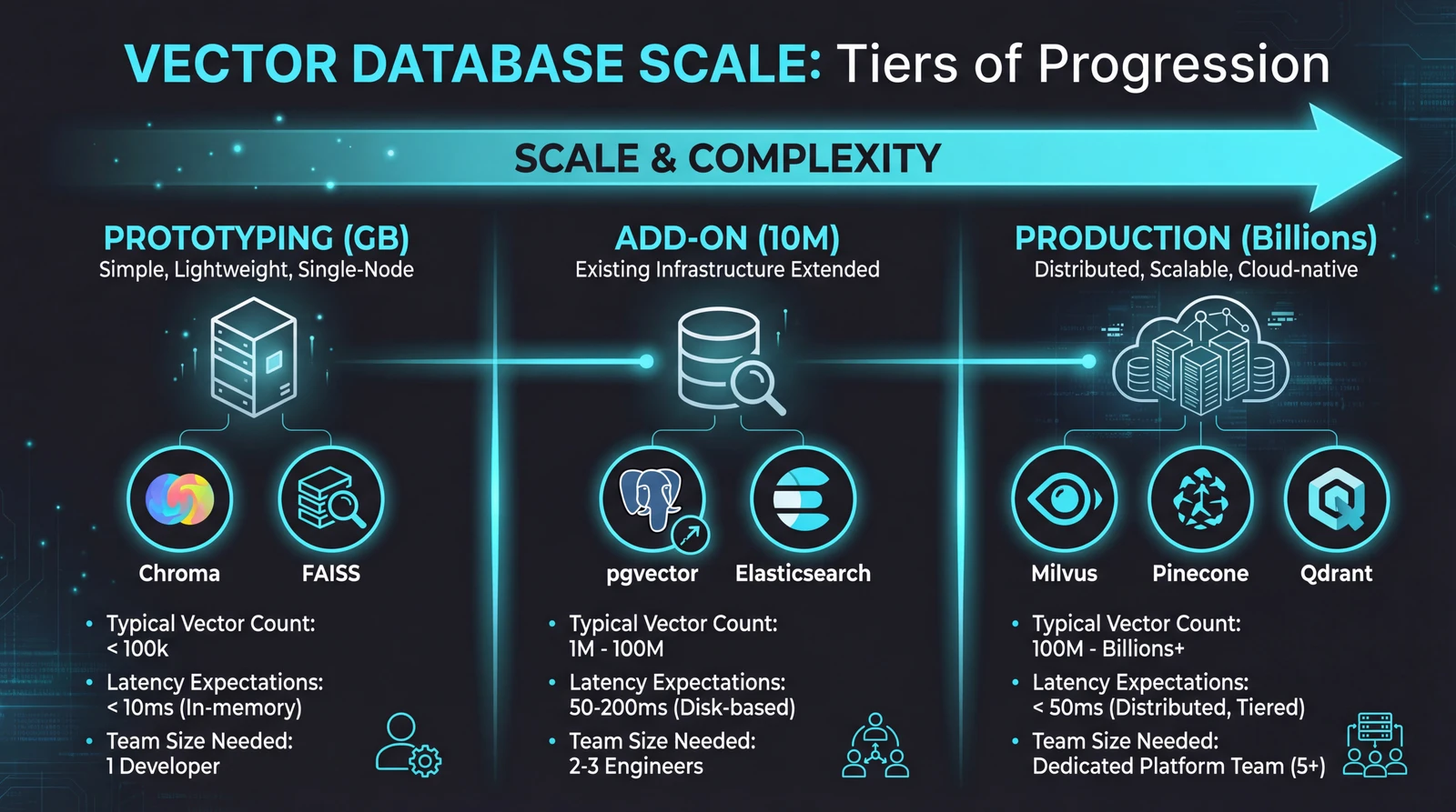
Tier 3: Production Vector Databases (TB Scale)
When you need billions of vectors with millisecond latency, 24/7 availability, and the ability to handle thousands of concurrent queries—this is the tier that matters.
Milvus is the open-source heavyweight. Built from the ground up for vector workloads, it uses a distributed architecture that scales horizontally. Segments are sharded across nodes, and the system handles rebalancing automatically. Zilliz Cloud offers a managed version.
Milvus consistently leads benchmarks for low-latency, high-throughput scenarios. Organizations like eBay, Shopify, and Walmart use it for production recommendation systems handling billions of vectors.
The complexity is proportional to the capability. Running Milvus at scale requires Kubernetes expertise, monitoring setup, and operational knowledge that many teams don't have. It's powerful, but it's not something you spin up in an afternoon.
Pinecone takes the opposite approach: fully managed, zero infrastructure. You get an API endpoint and don't think about servers, replication, or indexes. Pricing is per-vector and per-query.
The trade-off is control. You can't tune index parameters, can't run it in your own infrastructure, and can't inspect what's happening under the hood. For teams building AI products (not AI infrastructure), that's often the right trade-off.
Weaviate occupies an interesting middle ground. It excels at hybrid search—combining vector similarity with keyword matching and metadata filtering in single queries. Its modular architecture lets you plug in different embedding models and extend functionality.
Weaviate handles most RAG workflows well, with sub-100ms query times even on substantial datasets. But above 100 million vectors, it demands more memory and compute than alternatives. It's the right choice when your queries are complex (semantic search + filters + keyword matching), not when your queries are simple at massive scale.
Qdrant is written in Rust—which matters because Rust provides C++-level performance with strong memory safety guarantees. For a database that needs to be fast, stable, and handle heavy concurrent loads, that combination is valuable.
Qdrant's filtering is particularly efficient. Instead of pre-filtering (expensive) or post-filtering (inaccurate), it integrates filtering into the HNSW traversal itself. The result is single-pass searches that handle complex filter conditions without sacrificing speed.
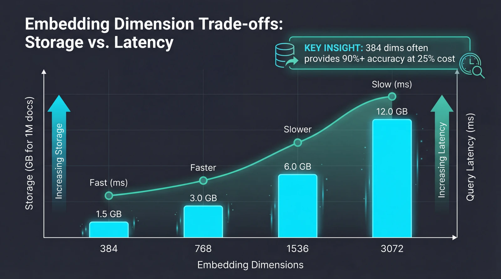
The Dimension Question
A decision you'll face early: how many dimensions should your vectors have?
OpenAI's text-embedding-3-large supports up to 3,072 dimensions. More dimensions mean more capacity to capture nuance. But the costs scale linearly:
- A million documents at 3,072 dimensions: ~12GB of vector storage
- The same documents at 384 dimensions: ~1.5GB
Computing similarity between 1,536-dimensional vectors is roughly 4x slower than 384-dimensional vectors. In practice, teams report that switching from 1,536 to 384 dimensions cut query latency in half and reduced database costs by 75%—often with no measurable drop in retrieval accuracy.
The newer embedding models support native dimension reduction. You can generate at 3,072 dimensions but request only the first 512 or 1,024, preserving most accuracy while reducing storage and improving speed.
The rule of thumb: Most business applications don't need maximum dimensions. Customer support queries, product documentation, and internal knowledge bases typically contain clear, well-structured information where 384-768 dimensions capture the semantic relationships users actually search for. Dense technical specifications with overlapping terminology might benefit from higher dimensions.
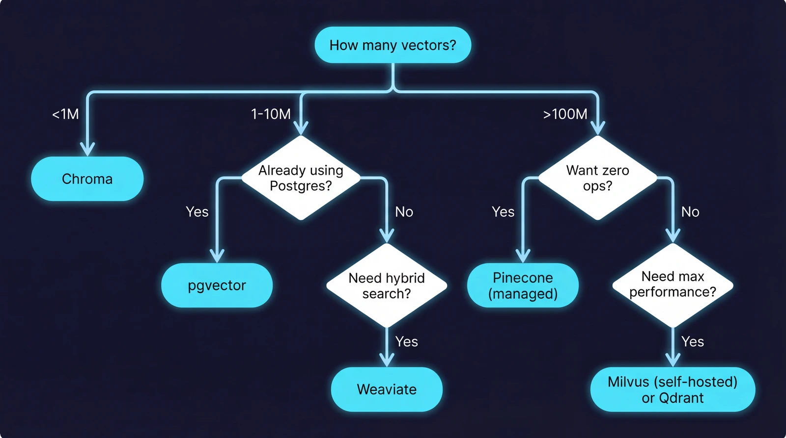
A Decision Framework
After working with various vector databases across projects, here's the framework I use:
| Your Situation | Recommendation |
|---|---|
| Prototyping, learning, under 1M vectors | Chroma |
| Already using PostgreSQL, under 10M vectors | pgvector |
| Need hybrid search (vectors + keywords + filters) | Weaviate |
| Billion-scale, performance-critical | Milvus |
| Want managed service, minimal ops | Pinecone or Qdrant Cloud |
| Rust ecosystem, filtering-heavy | Qdrant |
| Existing Elasticsearch investment | Elasticsearch (with realistic expectations) |
The meta-advice: Start with Chroma for prototyping. Validate your retrieval pipeline works before worrying about scale. Then migrate based on your actual requirements—which you'll only understand after building the prototype.
Most production systems don't need billion-vector capability. A surprisingly large number of successful RAG applications run on pgvector or Weaviate at scales that never stress those systems. Over-engineering the vector layer is a common mistake.
What's Next
The vector database market is projected to grow from roughly $2.5 billion in 2025 to over $10 billion by 2032. That growth is driven by AI adoption, but also by convergence—the line between "search engine" and "vector database" is blurring fast.
Elasticsearch adds vector capabilities. Vector databases add keyword search and metadata filtering. The endgame might be unified systems that handle all query types well, rather than specialized tools that excel at one thing.
For practitioners, the implication is clear: the tool you choose today may evolve into something different, and migrations between systems are becoming easier as APIs standardize. Focus on getting your retrieval pipeline working correctly, choose a database that handles your current scale with headroom, and stay flexible.
The embedding layer is where the value is. The storage layer, ultimately, is infrastructure.
Sources: